01-Beginning

ADT与DS

1. 抽象数据类型（Abstract Data Type，ADT）是计算机科学中具有类似行为的特定类别的数据结构的数学模型；或者具有类似语义的一种或多种程序设计语言的数据类型。抽象数据类型 = 数据模型 + 定义在该模型上的一组操作。

2. 数据结构（Data Structure）是计算机存储、组织数据的方式.数据结构 = 基于某种特定语言，实现ADT的一整套算法。

3. 对比：

   抽象数据类型ADT	数据结构DS
   抽象定义	具体实现
   一种定义	多种实现
   外部的逻辑特性	内部的表示和实现
   不考虑时间复杂度	与复杂度密切相关
   只考虑操作和语义	需要完整的算法实现
   不涉及数据的存储方式	要考虑数据的具体存储机制

4. 通俗易懂的例子：汽车驾驶员关心汽车的性能和驾驶表现；汽车制作者负责实现汽车的相应功能，二者通过汽车使用手册（说明书，ADT）来达成某种协议。

5. 另例：int n表示指定n属于int数据类型，其具有了int类型的某些特点，并支持相应的操作方法。但是，我们不用关心任务是如何完成的，而是关心能做什么。所以，我们需要将某些东西隐藏起来，不必详细说明实现过程。int float char Vector等都是抽象数据类型。

6. 抽象：不需详细说明实现过程的泛化操作称为抽象。即“抽取了过程的本质，而隐藏了实现的细节。

渐进分析

渐进符号

基础内容

Bachmann-Landau notation, also known as "Big-Oh" notation, abstracts away all constants in asymptotic analysis.

让$f(n),g(n)$为表示整数$n$的函数，我们使用如下的表示记号：

1. $f(n)\in O(g(n))$ if $\mathrm{\exists }c,n_0>0$ such that $f(n)\le c\cdot g(n)$ for all $n>n_0$.
2. $f(n)\in \mathrm{\Omega }(g(n))$ if $\mathrm{\exists }c,n_0>0$ such that $f(n)\ge c\cdot g(n)$ for all $n>n_0$.
3. $f(n)\in \mathrm{\Theta }(g(n))$ if both $f(n)\in O(g(n))$ and $f(n)\in \mathrm{\Omega }(g(n))$ hold.

对于Big-O和Big-Omega的严格版本，定义如下：

1. $f(n)\in o(g(n))$ if for every constant $c>0$, there exists an integer $n_0>0$ such that $f(n)<c\cdot g(n)$ for all $n>n_0$.
2. $f(n)\in \omega (g(n))$ if for every constant $c>0$, there exists an integer $n_0>0$ such that $f(n)>c\cdot g(n)$ for all $n>n_0$.

此外，我们还可以这样表示：

• $f(n)\in O(g(n))$ if $\underset{n\to \mathrm{\infty }}{lim}\frac{f(n)}{g(n)}\le c_1$ for some constant $c_1$ which is independent of n.

• $f(n)\in \mathrm{\Omega }(g(n))$ if $\underset{n\to \mathrm{\infty }}{lim}\frac{f(n)}{g(n)}\ge c_2$ for some constant $c_2$ which is independent of n.

• $f(n)\in \mathrm{\Theta }(g(n))$ if both $f(n)\in O(g(n))$ and $f(n)\in \mathrm{\Omega }(g(n))$ hold. (i.e. if $\underset{n\to \mathrm{\infty }}{lim}\frac{f(n)}{g(n)}=c$ for some constant $c$ which is independent of n.)

• $f(n)\in o(g(n))$ if $\underset{n\to \mathrm{\infty }}{lim}\frac{f(n)}{g(n)}=0$.

• $f(n)\in \omega (g(n))$ if $\underset{n\to \mathrm{\infty }}{lim}\frac{f(n)}{g(n)}=\mathrm{\infty }$.

注意：可以小写字母的符号推导到大写字母的符号，但是不能从某一个渐进符号的大写推出他的小写形式。

令$f(n)=2n^2+5n$，$g(n)=3n^2$，则有：

$$\underset{n\to \mathrm{\infty }}{lim}\frac{f(n)}{g(n)}=\underset{n\to \mathrm{\infty }}{lim}\frac{2n^2+5n}{3n^2}=\frac{2}{3}$$

令$c_1\in (\frac{2}{3},+\mathrm{\infty }),c=\frac{2}{3},c_2\in (0,\frac{2}{3})$即可。但是，不能说$f(n)\in o(g(n))$或$f(n)\in \omega (g(n))$。

增长速度

Function	Type of Growth
$1$	Constant Growth
${\log }^{\ast }n$	Iterative Logarithmic Growth
$\log \log n$	Twice Iterative Logarithmic Growth
$\log n$	Logarithmic Growth
${\log }^{k}n$ for some integer $k\ge 1$	Polylogarithmic Growth
$n^k$ for some $k\in (0,1)$	Sublinear Growth
$n$	Linear Growth
$n\log n$	Logarithmic-Linear Growth
$n{\log }^{k}n$ for some integer $k\ge 1$	Polylogarithmic-Linear Growth
$n^j{\log }^{k}n$ for some integer $j,k\ge 1$	Polylogarithmic-Polynomial Growth
$n^2$	Quadratic Growth
$n^3$	Cubic Growth
$n^k$ for some integer $k\ge 1$	Polynomial growth (General Situation)
$2^{{\log }^{k}n}$ for some $k>1$	Quasi-Polynomial Growth
$a^n$ for some $a>1$	Exponential Growth
$n!$	Factorial Growth
$n^n$	Super-Exponential Growth

计算技巧

• For any $\epsilon >0$, we have $\log n=o(n^{\epsilon })$.

• Striling Formula: $n!\sim \sqrt{2\pi n}{\left(\frac{n}{e}\right)}^n$.

  • For example, using Stirling Formula, we can prove that $\log n!=\mathrm{\Theta }(n\log n)$.

• Addition Rule:

  • If $f(n)\in O(g(n))$ and $h(n)\in O(k(n))$, then $f(n)+h(n)\in O(max(g(n),k(n)))$;
  • If $f(n)\in \mathrm{\Omega }(g(n))$ and $h(n)\in \mathrm{\Omega }(k(n))$, then $f(n)+h(n)\in \mathrm{\Omega }(min(g(n),k(n)))$.

• Composition Rule:

  • If $f(n)\in O(g(n))$ and $h(n)\in O(k(n))$, then $(f\circ h)(n)\in O(g\circ k)(n)$;
  • If $f(n)\in \mathrm{\Omega }(g(n))$ and $h(n)\in \mathrm{\Omega }(k(n))$, then $(f\circ h)(n)\in \mathrm{\Omega }(g\circ k)(n)$.

• L'Hôpital's Rule: Suppose $f(n)$ and $g(n)$ are both differentiable functions which satisfy L'Hôpital's Rule prerequisties, then

  $$$$$$$$$$$$$$Then,$$
  • If $L=-\mathrm{\infty }$, then $\underset{n\to \mathrm{\infty }}{lim}{\displaystyle \frac{f(n)}{g(n)}}=0$;
  • Otherwise, $\underset{n\to \mathrm{\infty }}{lim}{\displaystyle \frac{f(n)}{g(n)}}=2^L$.

  注意：这里不能使用$\underset{n\to \mathrm{\infty }}{lim}{\displaystyle \frac{\log A(n)}{\log B(n)}}$.

• Intergal Theorem: Let $f(x)>0$ be an increasing function or decreasing Riemann-integrable function over the interval $[1,+\mathrm{\infty })$, then

  $$\sum _{i=1}^{n}f(i)=\mathrm{\Theta }({\int }_1^{n}f(x)dx).$$

  if $f(x)$ is a decreasing function. Moreover, if $f(x)$ is an increasing function, the same is true, provided that $f(n)=O({\int }_1^{n}f(x)dx)$.

例题

• 判断$f(n)$是否为$O(g(n))$：

Question 1: Prove that $3n$ is $O(n^2)$.

Answer 1: $f(n)\le cg(n),\mathrm{\forall }n\ge n_0$. Let $n_0=1\Rightarrow c=3$. So statement$3n\le 3n^2,\mathrm{\forall }n\ge 1$ is true. Q.E.D.

• 判断$A(n)$和$B(n)$的时间复杂度关系（注意，不是所有的方程都能在渐进的意义下进行比较，如$f(n)=n^{1+\sin n}$）：

Question 2: Compute $\underset{n\to inf}{lim}\frac{A(n)}{B(n)}$ to find the relationship:

Answer 2:

• if it limits to 0: $A(n)\in O(B(n))$;
• if it limits to $\mathrm{\infty }$: $B(n)\in O(A(n))$;
• if it limits to non-zero values: $A(n)=\mathrm{\Theta }(B(n))$ (i.e. A(n) and B(n) has the same growth rate.);
• if it limits oscillationally, they are no relationship.

Question 3: Prove that $B(n)\in O(A(n))$, where $A(n)=2^n,B(n)=n^3$.

$$\begin{array}{rl}\underset{n\to \mathrm{\infty }}{lim}\frac{A(n)}{B(n)}& =\underset{n\to \mathrm{\infty }}{lim}\frac{2^n}{n^3}=\underset{n\to \mathrm{\infty }}{lim}\frac{2^n\cdot \ln 2}{3n^2}=\underset{n\to \mathrm{\infty }}{lim}\frac{2^n\cdot \ln 2\cdot \ln 2}{6n}\\ & =\underset{n\to \mathrm{\infty }}{lim}\frac{2^n\cdot \ln 2\cdot \ln 2\cdot \ln 2}{6}=\mathrm{\infty }\end{array}$$

which is to say, $B(n)$ is $O(A(n))$. $A(n)$ grows more than B(n).

参考资料

1. lecture2.pdf (jhu.edu)

2. bigO.pdf (csulb.edu)

3. ana-asymp-6up.pdf (chula.ac.th)

4. asymptotics - Are the functions always asymptotically comparable? - Computer Science Stack Exchange

递归式求解——代入法、递归树与主定理

递归式求解——代入法、递归树与主定理 - 知乎 (zhihu.com)

Master theorem (analysis of algorithms) - Wikipedia

从分治法到递归式

所谓分治法，就是把大问题分解成小问题，再把小问题的解合并成原问题的解。递归式则是用数学语言对这一过程的时间代价建模。如MergeSort的递推式：

$$T(n)=2T(n/2)+\mathrm{\Theta }(n),T(1)=\mathrm{\Theta }(1).$$

递归式的右侧通常由两部分组成，第一部分是分解后子问题的总代价，第二部分是分解和合并子问题的总代价。第一部分仍然是T的函数，第二部分则是实际的渐进复杂度。

以下有三种方法来求解递归式：代入法、递归树和主定理。

代入法

1. 我们需要先猜出解的形式，然后用数学归纳法证明该猜测是正确的。
2. 实例：假设猜测MergeSort的T解是$T(n)=O(n\log n)\to T(n)\le c\cdot n\log n,\mathrm{\exists }c\in \mathbb{R}.$ 然后猜测MergeSort $T(n)=\mathrm{\Omega }(n\log n)$, 若两者均正确，则MergeSort的T解为$T(n)=\mathrm{\Theta }(n\log n)$.
3. 代入法依赖于准确的猜测。

递归树

1. 把递归式逐层展开，直接就能得到一个树形结构。
2. 实例：$T(n)=3T(n/4)+\mathrm{\Theta }(n^2)$. 具体流程见网页链接。每层数据规模缩小为之前的四分之一，直到叶子结点数据规模为1，因此总层数为${\log }_{4}3$。右侧计算了每层所有结点的总代价：单个结点的代价乘以该层结点数量。最后一层单个结点的代价为常数，结点数量$3^{{\log }_{4}n}=n^{{\log }_{4}3}$，记作$\mathrm{\Theta }(n^{{\log }_{4}3})$。然后对几何级数求和（放缩、舍去低阶项）。
3. 有些情况下，利用递归树计算精确的解会稍有困难，但不妨碍我们做出一个合理的猜测，然后进一步用代入法验证该猜测。

主方法

代入法和递归树法各有缺点，前者需要一个准确的猜测，后者需要画出递归树并推导结果。而大部分递归式解的形式都是一样的。我们也许可以通过对递归式分类，按照某种规则直接写出最终的解。

若分治法每一次都均分数据时，递归式具有如下一般的形式：

$$T(n)=\{\begin{array}{ll}aT(n/b)+f(n)& \text{ if }n\ge d\\ \mathrm{\Theta }(1)& \text{ if }n<d\end{array}$$

这里，a是一个正整数，表示每次分治，问题被分解为a个子问题;

b 是一个大于1的整数，表示每次分治，问题规模缩小为之前的${\displaystyle \frac{1}{b}}$.

*f(n)*是渐进正函数，表示分解和合并的代价。

用递归树找统一解，Total为所有节点的总代价：

$T(1)=\mathrm{\Theta }(1)$为基本操作所花费的时间。化简后，有：

$$T(n)=n^{{\log }_{b}a}\cdot T(1)+\sum _{j=0}^{{\log }_{b}n-1}{a}^{j}f\left(n/b^j\right)$$

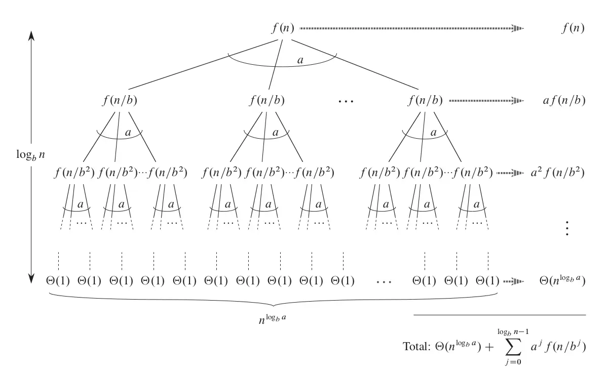
下面有三种情况，按照两个和项的大小进行分类，即比较$f(n)$和$n^{{\log }_{b}a}$的大小：

1. 若$f(n)$渐进小于$n^{{\log }_{b}a}$.，即认为$\mathrm{\exists }ϵ>0,s.t.f(n)=O(n^{{\log }_{b}a-ϵ})$成立时，有$T(n)$为$\mathrm{\Theta }(n^{{\log }_{b}a})$.

If $f(n)$ is $O(n^{{\log }_{b}a-\epsilon })$, then $T(n)$ is $\mathrm{\Theta }(n^{{\log }_{b}a})$.

2. 若$f(n)$和$n^{{\log }_{b}a}{\log }^{k}n$相等$(k\ge 0)$，则$T(n)=\mathrm{\Theta }(n^{{\log }_{b}a}{\log }^{k+1}n)$.

If $f(n)$ is $\mathrm{\Theta }(n^{{\log }_{b}a}{\log }^{k}n\mathbb{R})$, then $T(n)$ is $\mathrm{\Theta }(n^{{\log }_{b}a}{\log }^{k+1}n\mathbb{R})$.

3. 若$f(n)$渐进大于$n^{{\log }_{b}a}$，且对于$\delta$<1和所有足够大的n有$af(n/b)\le \delta f(n)$， 则有$T(n)=\mathrm{\Theta }(f(n))$.

If $f(n)$ is $\mathrm{\Omega }\left(n^{{\log }_{b}a+\epsilon }\mathbb{R}\right)$ , then T(n) is $\mathrm{\Theta }(f(n))$ , provided a $f(n/b)\le \delta f(n)$ for some $\delta <1$ .

实例：$T(n)=9T(n/3)+n,a=9,b=3,f(n)=n,n^{{\log }_{b}a}=n^2$, $f(n)<\mathrm{\Theta }(n^2)$, 故$T(n)=\mathrm{\Theta }(n^2)$.

必须注意，主定理第三条要检查其是否满足附加条件。并非所有满足上面形式的式子都可以使用主定理来进行判定。如$T(n)=2T(n/2)+n\log n$, 不满足上述附加条件，故只能使用递归树求解。求解过程如下：

$$T(n)=2T(n/2)+n\log n$$

对于该式，有 $a=2,b=2,f\left(n\mathbb{R}\right)=n\log n$ ，此时 $n^{lo{g}_{b}a}=n^{lo{g}_{2}2}=n$ 。显然， $f(n\mathbb{R})=n\log n$ 渐进大于 $n$ ，应考虑主定理的第三种情况。将其带入附加条件，得

$$\begin{array}{rl}2\frac{n}{2}\lg \frac{n}{2}& \le cn\lg n\\ \lg n-1& \le c\lg n\\ (1-c)\lg n& \le 1\end{array}$$

当 $c\ge 1$ 时，该式恒成立。但附加条件要求 $c<1$ ，因此该式不能使用主方法的第三种情况。结果为$T(n)=\mathrm{\Theta }(n{\log }^{2}n)$.

令解：带入方法2可求解。

特别内容

1. 对于任意一个符合主定理格式的递归式，如果它满足情况三中的正则条件，那么它一定满足$f(n)-\mathrm{\Omega }(n^{{\log }_{b}a+ϵ})$, 而反过来不可推出。
2. 另一个例子：求解递推方程$T(n)=T(n/3)+T(2n/3)+n$. 这个递归树的树叶不在同一层上面。此时，应从最坏的情况出发，考虑最长的路径。那么这个递归树一共有$k={\log }_{3/2}n$层。（2n/3一侧的路径最长，每走一步，问题规模会变成原来的2/3.）而每一层节点的数值之和为O(n)，从而有：$T(n)=O(n{\log }_{3/2}n)=O(n\log n)$.

Wikipedia上的主定理——Generic Form

1. The master theorem always yields asymptotically tight bounds to recurrences from divide and conquer algorithms that partition an input into smaller subproblems of equal sizes, solve the subproblems recursively, and then combine the subproblem solutions to give a solution to the original problem. The time for such an algorithm can be expressed by adding the work that they perform at the top level of their recursion (to divide the problems into subproblems and then combine the subproblem solutions) together with the time made in the recursive calls of the algorithm. If $T(n)$ denotes the total time for the algorithm on an input of size $n$ and $f(n)$ denotes the amount of time taken at the top level of the recurrence then the time can be expressed by a recurrence relation that takes the form:

2. Here $n$ is the size of an input problem, $a$ is the number of subproblems in the recursion, and $b$ is the factor by which the subproblem size is reduced in each recursive call (b>1). Crucially, $a$ and $b$ must not depend on $n$. The theorem below also assumes that, as a base case for the recurrence, $T(n)=\mathrm{\Theta }(1)$ when $n$ is less than some bound $\kappa >0$, the smallest input size that will lead to a recursive call.

3. Recurrences of this form often satisfy one of the three following regimes, based on how the work to split/recombine the problem $f(n)$ relates to the critical exponent $c_{crit}={\log }_{b}a$.

   1. Case 1:

      • Description: Work to split/recombine a problem is dwarfed by subproblems. (I.e. the recursion tree is leaf-heavy.)

      • Condition on $f(n)$ in relation to $c_{crit}$, i.e. ${\log }_{b}a$: When $f(n)=O(n^c)$ where $ c<c_{crit}$. (upper-bounded by a lesser exponent polynomial)

      • Master Theorem bound: then $T(n)=\mathrm{\Theta }(n^{c_{crit}})$. (The splitting term does not appear; the recursive tree structure dominates.)

      • Notational examples: If $b=a^2$ and $f(n)=O(n^{1/2-ϵ})$, then $T(n)=\mathrm{\Theta }(n^{1/2})$.

        描述：拆分/重组问题的工作与子问题相形见绌。（即递归树的叶子过多）

        $f(n)$和${\log }_{b}a$的关系：当$f(n)=O(n^c)$时，其中$c<{\log }_{b}a$。（上界为小指数多项式）

        主定理的约束条件：$T(n)=\mathrm{\Theta }(n^{c_{crit}})=T(n)=\mathrm{\Theta }(n^{{\log }_{b}a})$。（递归树占主导地位，而未出现拆分项。）

   2. Case 2:

      1. Description: Work to split/recombine a problem is comparable to subproblems.

      2. Condition on $f(n)$ in relation to $c_{crit}$, i.e. ${\log }_{b}a$: When $f(n)=\mathrm{\Theta }(n^{c_{crit}}{\log }^{k}n)$ for a $k\ge 0$ (rangebound by the critical-exponent polynomial, times zero or more optional $\log s$)

      3. Master Theorem bound: then $T(n)=\mathrm{\Theta }(n^{c_{crit}}{\log }^{k+1}n\mathbb{R})$ (The bound is the splitting term, where the log is augmented by a single power.)

      4. Notational examples: If $b=a^2$ and $f(n)=\mathrm{\Theta }(n^{1/2})$, then $T(n)=\mathrm{\Theta }(n^{1/2}\log n)$; If $b=a^2$ and $f(n)=\mathrm{\Theta }(n^{1/2}\log n)$, then $T(n)=\mathrm{\Theta }(n^{1/2}{\log }^{2}n)$.

         描述：拆分/重组问题的工作与子问题相当。

         $f(n)$和${\log }_{b}a$的关系：当 $f(n)=\mathrm{\Theta }(n^{c_{crit}}{\log }^{k}n)$时，其中$k\ge 0$。（界被${\log }_{b}a$所限，乘以零或可选的$\log s$）

         主定理的约束条件：$T(n)=\mathrm{\Theta }(n^{c_{crit}}{\log }^{k+1}n\mathbb{R})$。（界值为拆分项，对数的次数增加1。）

   3. Case 3:

      1. Description: Work to split/recombine a problem dominates subproblems. (I.e. the recursion tree is root-heavy.)

      2. Condition on $f(n)$ in relation to $c_{crit}$, i.e. ${\log }_{b}a$: When $f(n)=\mathrm{\Omega }(n^c)$ where $c>c_{crit}$. (lower-bounded by a greater exponent polynomial)

      3. Master Theorem bound: this doesn't necessarily yield anything. Furthermore, if $af\left(\frac{n}{b}\mathbb{R}\right)\le kf(n)$ for some constant $k<1$ and sufficiently large $n$ (often called the regularity condition) then the total is dominated by the splitting term $f(n)$: $T\left(n\mathbb{R}\right)=\mathrm{\Theta }(f(n)\mathbb{R})$.

      4. Notational examples: If $b=a^2$ and $f(n)=\mathrm{\Omega }(n^{1/2+ϵ})$ and the regularity condition holds, then $T(n)=\mathrm{\Theta }(f(n))$.

         描述：拆分/重组问题的工作远胜于子问题。（即递归树的根过多）

         $f(n)$和${\log }_{b}a$的关系：当$f(n)=O(n^c)$时，其中$c>{\log }_{b}a$。（下界为大指数多项式）

         主定理的约束条件：这不一定有结果。若$\mathrm{\exists }k<1$和一个很大的$n$（规则性条件），有$af\left({\displaystyle \frac{n}{b}}\mathbb{R}\right)\le kf(n)$，则结果由拆分项$f(n)$主导，$T\left(n\mathbb{R}\right)=\mathrm{\Theta }(f(n)\mathbb{R})$。

A useful extension of Case 2 handles all values of $k$:

Case	Condition on $f(n)$ in relation to $c_{crit}$, i.e. ${\log }_{b}a$	Master Theorem bound	Notational examples
2a	When $f(n)=\mathrm{\Theta }(n^{c_{crit}}{\log }^{k}n)$ for any $k>-1$	... then $T(n)=\mathrm{\Theta }(n^{c_{crit}}{\log }^{k+1}n\mathbb{R})$ (The bound is the splitting term, where the log is augmented by a single power.)	If $b=a^2$ and $f(n)=\mathrm{\Theta }(n^{1/2}/{\log }^{1/2}n)$, then $T(n)=\mathrm{\Theta }(n^{1/2}{\log }^{1/2}n)$.
2b	When $f(n)=\mathrm{\Theta }(n^{c_{crit}}{\log }^{k}n)$ for $k=-1$	... then $T(n)=\mathrm{\Theta }(n^{c_{crit}}\log \log n\mathbb{R})$ (The bound is the splitting term, where the log reciprocal is replaced by an iterated log.)	If $b=a^2$ and $f(n)=\mathrm{\Theta }(n^{1/2}/\log n)$, then $T(n)=\mathrm{\Theta }(n^{1/2}\log \log n)$.
2c	When $f(n)=\mathrm{\Theta }(n^{c_{crit}}{\log }^{k}n)$ for any $k>-1$	... then $T(n)=\mathrm{\Theta }\left(n^{c_{crit}}\mathbb{R}\right)$ (The bound is the splitting term, where the log disappears.)	If $b=a^2$ and $f(n)=\mathrm{\Theta }(n^{1/2}/{\log }^{2}n)$, then $T(n)=\mathrm{\Theta }(n^{1/2})$.

摊还分析

摊还分析（Amortized Analysis）是一种确定数据结构操作成本的高级策略，它可以找出在一系列操作中，平均每个操作的时间复杂度。摊还分析并不关注每个操作的实际成本，而是关注操作序列的平均成本。参见数据结构时间复杂度的摊还分析（均摊法）之一：基础

摊还分析有三种常见的方法：

1. 聚集分析（Aggregate Analysis）：这种方法将一系列操作的总成本分摊到每个操作上。例如，如果我们有一个可以在O(1)时间内完成插入的数据结构，但是每10次插入需要花费O(n)的时间来重新整理，那么聚集分析会将这个O(n)的成本分摊到这10次插入上，得出平均每次插入的成本是O(1)。

2. 记账法（Accounting Method）：这种方法通过给便宜的操作“存款”，然后在昂贵的操作时“取款”来进行分析。便宜的操作存款的额度会超过它们的实际成本，这个额外的成本就是为了在后面昂贵的操作时使用。

3. 势能法（Potential Method）：这种方法将数据结构看作是一个物理系统，定义一个“势能”函数来度量系统的“能量”。便宜的操作会增加系统的势能，昂贵的操作会消耗势能。通过势能的变化，我们可以计算出操作的摊还成本。

例如，动态数组（Vector）等可以使用聚合分析；二叉堆的插入操作和栈的入栈、出栈和遍历出栈可以使用记账法；斐波那契堆删除的最小元素操作可以使用势能法。